Testing optimisation algorithms: Part II - Implementing objective function in R

In Part I I presented the reasons I'm interested in optimisation, and gave a mathematical statement of the example constrained optimisation problem I will solve. In this post, I am going to present two practical implementation algorithms, coded in R. I'll also present an R function for visualising the resultant circles.

The code can be found at the end of this post, it's fairly well commented, so just some general comments first:

Most optimisation functions take a single vector of parameter values as an argument. This is a bit unwieldy for our problem, since we have N triplets of x,y and r. Here I arbitrarily define a parameter vector z, of length 3*N and split it up (consistently) into vectors for x, y and r.

R has a convenient combinatorics facility, so I use that to generate a unique list of all possible circle pairs to optimise the calculations required for constraint g5.

I'm using function closures here to avoid defining global variables. In R, a function closure is a function which returns another function but with its own environment for storing variables etc., which can be initialised within the outer function before returning the inner function. For example, I have created a function createObj which initialises the number of circles N, and the rectangle dimensions (W and H), generates a unique list of circle pairs (cpairs) and creates a function newObj which only depends on z, but nevertheless has access to private copies of N, W, H and clist.

Here, constraints are embedded into the objective function. A numerical value is associated with constraint violation and is subtracted from the objective function we are trying to maximise. There are two alternative versions of the objective function closures in the code below: createObj is "soft", the constraint violation values are the sum of the square of the magnitude of violations, createHardObj is "hard", any single violated constraint, no matter how small, returns in an area of -Infinity. In the first case, a derivative based algorithm will always be able to figure out a path towards satisfying constraints if it finds itself in a region where they are violated, but small violations may be tolerated in the final solution. In the latter case, all constraints must be completely obeyed, but on the other hand, there are no hints about how to improve from an invalid set of parameters.

The drawCircles function can plot circles to screen, or in vector graphics format (to a .pdf for example). Here are some outputs generated with this function (initial guess on left, optimised result on right):

CirclePackingCircles

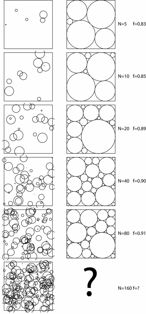
Finally, the optimisation routine presented here just uses the L-BFGS-B method which is a pretty good, bounded, derivative-based optimiser, which is made available within the optim function which is standard in R installations (it's part of the core). It's fairly slow for more than 100 circles, and the results are not perfect, as circles are often forced to the edge of the box with negligble radii. Nevertheless, it's a good start.


  1
  2
  3
  4
  5
  6
  7
  8
  9
 10
 11
 12
 13
 14
 15
 16
 17
 18
 19
 20
 21
 22
 23
 24
 25
 26
 27
 28
 29
 30
 31
 32
 33
 34
 35
 36
 37
 38
 39
 40
 41
 42
 43
 44
 45
 46
 47
 48
 49
 50
 51
 52
 53
 54
 55
 56
 57
 58
 59
 60
 61
 62
 63
 64
 65
 66
 67
 68
 69
 70
 71
 72
 73
 74
 75
 76
 77
 78
 79
 80
 81
 82
 83
 84
 85
 86
 87
 88
 89
 90
 91
 92
 93
 94
 95
 96
 97
 98
 99
100
101
102
103
104
105
106
107
108
109
110
111
112
113
114
115
116
117
118
119
120
121
122
123
124
125
126
127
128
129
130
131
132
133
###########
# Optimum circle packing in R
###########

# Function closure, sets up list of possible combinations
# and returns objective function
createObj<-function(N,W,H){

print("Generating combinations...")
# Generate all possible circle pairings
cpairs=data.frame(t(combn(1:N,2)))
colnames(cpairs)=c("A","B")
print("Combinations complete.")

return({
	newObj<-function(z){
		# This vector is split up into triplets of x,y,r 
		# z[1],z[2],z[3] -> x1,y1,r1
		x=z[1:N*3-2]
		y=z[1:N*3-1]
		r=z[1:N*3-0]

		res=0
		# Some linear inequality constraints to be satisfied
		c1=x+r-W # <0	
		c2=y+r-H # <0
		c3=r-x # <= 0
		c4=r-y # <=0
		# Many nonlinear inequality constraints
		c5=r[cpairs$A]+r[cpairs$B]-sqrt((x[cpairs$A]-x[cpairs$B])^2+(y[cpairs$A]-y[cpairs$B])^2) # <=0

		c1=c1[c1>0]
		c2=c2[c2>0]
		c3=c3[c3>0]
		c4=c4[c4>0]
		c5=c5[c5>0]
		constraints=c(c1,c2,c3,c4,c5)
		if(length(constraints)>0){
			constraints=constraints^2
			res=res-sum(constraints)
		}
		
		# Actual objective function (fraction of area covered)
		res=res+(pi*sum(r^2))/(W*H)
	
		return(-1*res)
	}
})
}

# Function closure, sets up list of possible combinations
# and returns objective function
createHardObj<-function(N,W,H){

print("Generating combinations...")
# Generate all possible circle pairings
cpairs=data.frame(t(combn(1:N,2)))
colnames(cpairs)=c("A","B")
print("Combinations complete.")

return({
	newHardObj<-function(z){
		# This vector is split up into triplets of x,y,r 
		# z[1],z[2],z[3] -> x1,y1,r1
		x=z[1:N*3-2]
		y=z[1:N*3-1]
		r=z[1:N*3-0]

		res=0
		# Some nonlinear inequality constraints to be satisfied
		if(FALSE%in%(x+r<W)) res = Inf
		if(FALSE%in%(y+r<H)) res = Inf
		if(FALSE%in%(x-r>=0)) res = Inf
		if(FALSE%in%(y-r>=0)) res = Inf
		# Many nonlinear inequality constraints
		if(FALSE%in%(((x[cpairs$A]-x[cpairs$B])^2+(y[cpairs$A]-y[cpairs$B])^2)>=(r[cpairs$A]+r[cpairs$B])^2)) res = Inf
	
		# Actual objective function (fraction of area covered)
		res=res+(pi*sum(r^2))/(W*H)
	
		return(-1*res)
	}
	})
}

# Draw circles (centres and radii speficied in df)
# within a bounding rectangle (width * height)
drawCircles<-function(df,width,height,colour="black",pdfName=NULL){
	if(is.null(pdfName)){
		graphics.off()
		dev.new(width=7, height=7*height/width)
	}else{
		pdf(pdfName,width=7,height=7*height/width)
	}
	maxdim=max(width,height)
	width=width/maxdim
	height=height/maxdim
	df=df/maxdim
	# Change to coordinate system based on centre of rectangle
	df$x=df$x-width/2
	df$y=df$y-height/2
	# Draws circles on a square
	par(plt=c(0,1,0,1))
	plot(NULL,xlim=c(-width/2,width/2),ylim=c(-height/2,height/2),axes=FALSE,xaxt='n',yaxt='n',ann=FALSE)
	symbols(df$x,df$y,circles=df$r,fg=colour,bg=NA,add=TRUE,inches=FALSE) 
	rect(-width/2,-height/2,width/2,height/2)
	if(!is.null(pdfName)) dev.off()
}

# Number of circles and dimensions of bounding rectangle 
N=13; W=10; H=10

# Create objective function
obj=createObj(N,W,H)

# Lowest acceptable values for dimensions or radii (x,y,r) is zero
low=rep(0,3*N)
# x can go as high as W, y as high as H
# The biggest allowable circle radius is the smaller of W and H
up=rep(c(W,H,min(W,H)),N)
# Initial guess (random circle coordinates and radii)
z=rep(0,3*N)
z[1:N*3-2]=runif(N,0,W)
z[1:N*3-1]=runif(N,0,H)
z[1:N*3-0]=runif(N,0,0.1*min(W,H))

out=optim(par=z,fn=obj,method="L-BFGS-B",lower=low,upper=up,control=list(maxit=2000))
cat("Fractional area:",-1*out$value)

z=as.numeric(out$par)
x=z[1:N*3-2]; y=z[1:N*3-1]; r=abs(z[1:N*3-0])
dfA=data.frame(x=x,y=y,r=r)
drawCircles(dfA,W,H)

Comments

Reformatted code

I just reformatted the code above using the very excellent http://www.hilite.me/ website. Much more readable!