Oscillations

Last week a colleague asked for advice on how to estimate the frequency and amplitude of an oscillating signal. My initial response was to suggest reading the data into R, using the spectrum function to estimate the spectral density of the time series, taking the maximum as a good initial guess for the frequency of oscillation and using that initial guess to fit a sinusoid model to the data by least squares. I suggested trying to fit the rather gruesome "monthly deaths from bronchitis, emphysema and asthma in the UK, 1974–1979" dataset ldeaths which is embedded in R, and referred to as an example in the spectrum documentation.

On reflection, I think that this was a terrible example to give, since the ldeaths time-series is nice and regular. One thing I've learned from 10 years of working with biological data is that they are almost never regular or well-behaved. Therefore analysing this dataset is likely to be misleading. Many statistical tools assume regular datasets.

The alternative, more realistic example R workflow I now recommend (including the generation of a realistic, synthetic, example dataset) can be seen at the bottom of this post. Here is an example output:

Oscillating dataset and fitted models

While writing this, I remembered that way back in 2000 I ran a website which described solving this very problem as an example of using the Newton-Rhapson method for multi-dimensional optimisation. The tools I used then are different, but the two main principles are the same: 1) fit a model to the data for a robust estimate of frequency & amplitude and 2) take care to generate good initial guesses for parameter values if you want a sensible fit.

If we wanted to test for the significance of differences between frequency estimates generated from different datasets, without multiple experimental repeats, the problem becomes more interesting. In that case I would recommend using JAGS and rjags to infer distributed parameter values for the same model (with an added error model).


 1
 2
 3
 4
 5
 6
 7
 8
 9
10
11
12
13
14
15
16
17
18
19
20
21
22
23
24
25
26
27
28
29
30
31
32
33
34
35
36
37
38
39
40
41
42
43
44
45
46
47
48
49
50
51
52
53
54
55
56
57
58
59
60
61
62
63
64
65
66
67
68
69
############################
# Generate best estimate for frequency and amplitude given irregular timeseries
# displaying oscillations by fitting a sinusoidal model.
############################

### Define sinusoid model
mod=function(A,f,c,p,t) A*sin(2*pi*f*t+p)+c

### Use model to generate a synthetic irregular time-series (with noise)
### For a real problem, replace this section with actual data!
# True paramter values
Atrue=5; ftrue=1/30; ctrue=20; ptrue=0
# Random simulation of irregular observation schedule
expt=sort(sample(0:100,50,replace=FALSE))
# Generate realistic dataset (irregular observation times and observations with error)
df=data.frame(time=expt,obs=mod(Atrue,ftrue,ctrue,ptrue,expt)+rnorm(length(expt),mean=1,sd=2))

### Estimate frequency of data by simulating a regular time-series
# Construct interpolating function for observed data
intf=approxfun(df$time,df$obs)
# Simulate a regular measurement frequency
mfreq=2
# Create regularly spaced time-series
regtimes=min(df$time)+mfreq*(0:((max(df$time)-min(df$time))/mfreq))
regobs=intf(regtimes)
# Generate and plot frequency spectrum for regular time-series
spec=spectrum(regobs,plot=TRUE)
# Extract the fundamental frequency
fguess=spec$freq[which.max(spec$spec)]
# Convert units from measurent frequency original units
fguess=fguess/mfreq

### Estimate other paramters
# Estimate amplitude as half range of observations
Aguess=(max(df$obs)-min(df$obs))/2
# Estimate offset as mean of observations
cguess=mean(df$obs)
# Estimate the phase as 
pguess=asin((df$obs[1]-cguess)/Aguess)-2*pi*fguess*df$time[1]

### Fit model to data
# Objective function (sum of squared difference between model and observations)
obj<-function(z){
	A=z[1]; f=z[2]; c=z[3]; p=z[4];
	return(sum((mod(A,f,c,p,df$time)-df$obs)**2))
}
# Optimisation
# Approximate sampling frequency (to avoid Nyquist limit)
sfreqest=length(df$time)/max(df$time)
lowerlim=c(0,0,-Inf,0)
upperlim=c(Inf,2*sfreqest,Inf,2*pi)
params=optim(c(Aguess,fguess,cguess,pguess),obj,lower=lowerlim,upper=upperlim,method="L-BFGS-B",control=list(maxit=10000))$par
Aopt=params[1]; fopt=params[2]; copt=params[3]; popt=params[4]
Apercent=100*(Atrue-Aopt)/Atrue; fpercent=100*(ftrue-fopt)/ftrue; cpercent=100*(ctrue-copt)/ctrue; ppercent=100*(ptrue-popt)/(2*pi)
report=paste("% Diffs: A:",signif(Apercent,3),"f:",signif(fpercent,3),"c:",signif(cpercent,3),"p:",signif(ppercent,3))

# Inspect goodness of fit
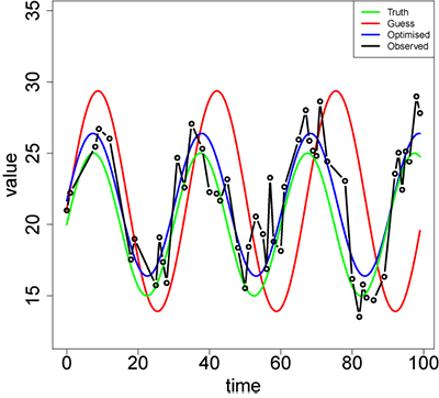
#pdf("Oscillations.pdf",width=8,height=8)
	plot(NULL,,xlim=c(min(df$time),max(df$time)),ylim=c(0.9*min(df$obs),1.2*max(df$obs)),type="n",xlab="time",ylab="value",main=report,cex.lab=2,cex.axis=2)
	curve(mod(Aguess,fguess,cguess,pguess,x),min(df$time),max(df$time),add=TRUE,col="red",lwd=3,,n=1001)
	curve(mod(Aopt,fopt,copt,popt,x),min(df$time),max(df$time),add=TRUE,col="blue",lwd=3,n=1001)
	curve(mod(Atrue,ftrue,ctrue,ptrue,x),min(df$time),max(df$time),add=TRUE,col="green",lwd=3,n=1001)
	points(df$time,df$obs,type="b",lwd=3)
	legend("topright",c("Truth","Guess","Optimised","Observed"),lwd=3,col=c("green","red","blue","black"))
#dev.off()
# Generate a small report
res=data.frame(A=c(Atrue,Aguess,Aopt),f=c(ftrue,fguess,fopt),c=c(ctrue,cguess,copt),p=c(ptrue,pguess,popt))
rownames(res)=c("Truth","Guess","Optimised")
print(res)

Comments

Avoiding Nyquist sampling problems...

Glyn Nelson pointed out that on occasional runs of the script above the optimised frequency came out far too high. To get around this, I've changed the script to use constrained optimisation (instead of the default optimiser in the optim function) guesstimating the sampling frequency and constraining the fitted frequency to be less than twice that, in accordance with the Nyquist sampling theorem. The script still gives erroneous results occasionally. Around 1% of the time it chooses a frequency of zero for example. This could be dealt with by increasing the lower limit for f a small amount above zero, but since the definition of "small" in this case is problem-specific, I will leave the limit as it is.

What about oscillations that drift in phase?

Darren Wilkinson gave a nice talk the other day which reminded me that there is another problem with oscillatory data that I haven't mentioned here. A closed, stochastic, dynamical, oscillatory system will have irregular peaks and troughs as well as noisy local values. In other words, frequency itself could also have significant variance. In this case, a single sinusoid curve (even with an added error model) will not capture this behaviour sensibly and it is usually best to formulate a stochastic model of the mechanisms underlying the oscillation which will capture this behaviour naturally. Parameter inference for such a model is more difficult, however.

By closed I mean a system which is not susceptible to external forcing, so system dynamics are entirely internal. However many biological systems are susceptible to external forcing. These include the yearly growth cycles of annual plants (growth in biomass: leaves and fruit), yearly weather cycles (temperature, moisture availability, daylength), daily or circadian cycles (largely closed but entrained by light, temperature, waking-sleeping).

The existence of such external forces acting to regularly correct your system will probably remove the necessity for developing a stochastic model, but on the other hand, if they have a significant effect on the system in question, they too could usefully be modelled and observed.

Reformatted code

I just reformatted the code above using the very excellent http://www.hilite.me/ website. Much more readable!