13 April 2017

Image analysis in Python: locating & visualising areas of an image that are in sharp focus

In this post I’ll demonstrate how to locate and highlight the areas of any digital image that are in focus. In microscopy and macro photography, being able to identify image segments that are in focus is important because of the narrow depth-of-field achievable using wide apertures. If you need to construct a high resolution image of a very small subject, you may have to capture a stack of several images (often called a z-stack), each focussed on a different slice of the subject. You are then left with the problem of how to combine these images into one composite image with the entire subject in focus. The first steps in generating a composite image from such a stack of images is constructing a quantitative measure of focus and using it to identify segments in each image in the stack that are in focus.

Image analysis in Python is fun

I have written the short piece of code for this analysis in Python, using the Python Imaging Library (PIL), NumPy and SciPy.

I have really enjoyed using Python for image analysis in the past. It can be an extremely powerful image analysis tool when combined with NumPy & SciPy (and also OpenCV, however I will not use OpenCV in this example). Python is a general purpose programming language, with a clean, syntax that is easy to read and learn. I often wish that it had been the first language I had been introduced to when I first started to learn programming; it’s so quick and easy to get to the stage where you can make the computer carry out useful tasks! The fact that it is general purpose means that it can be integrated into almost any computational workflow with ease.

Alternatives to Python

However, Python does have some drawbacks for scientific computing. In particular, it requires installation of a lot of additional packages (e.g. NumPy and SciPy above) before you can carry out really heavy computation. Once installed, these are powerful and easy to use, however, the default package management systems in Python leave a lot to be desired. They have improved in the past couple of years, but in 2017, beginners still struggle with installing packages across all operating systems. For example, installing additional Python packages on 64-bit Windows machines remains a bit of a minefield.

Julia seems to be a more modern, easier alternative to Python for image analysis. It is designed for fast, array-based programming, and has been built around an excellent package management system, based on GitHub. Julia is also designed with parallel programming in mind, unlike Python. I intend to explore this alternative more fully soon.

Some biological scientists love to use a Java-based software called ImageJ for image analysis. ImageJ is primarily based around a graphical user interface (GUI). I strongly prefer to avoid carrying out analyses using GUIs as they cannot be easily automatically incorporated into computational workflows. Code-based analysis, on the other hand, can easily be automated, can be built into robot-based lab workflows and can be shared and published unambiguously, much like laboratory protocols.

Other scientists enjoy using Matlab for image analysis work. Matlab is closed, proprietary software which is really unsuitable for publishing and sharing code (prospective users must own an expensive license before they can try your code out). Dealing with proprietary licenses limits the range of people that you can share your work with as well as the number of actual machines that you can work on. These days there are plenty of great alternatives (e.g. Python, as we will see in this example). We don’t have to use proprietary software for scientific computing anymore.

Code for finding focus

First we import some Python packages to extend Python’s capabilities and allow us to do some image analysis. I assume that you have already successfully installed these on your machine. We import the Image module from the PIL package, the ndimage module from scipy and we import the entire numpy package and give it a shorter name: np.

from PIL import Image
from scipy import ndimage
import numpy as np

Next we define the name of an RGB image file that we will read from Python’s working directory. If the image is exceptionally high resolution, you might run into memory issues later on. If Python returns an error that mentions memory, just try a smaller image. We also define a variable sigma, which we will use later to define a sort of search space for focus. Smaller values of sigma will result in more sharply defined focus areas.

fname = "reddoor.jpg"
sigma = 2.0

We open the image, and store it in a variable named im, then convert im into a three-dimensional (see below) numerical array (arr). We will also need an overall value for intensity at each pixel location. To create that, we convert the colour RGB image into a greyscale image (imbw), and use that to create the corresponding two-dimensional array version (arrbw) of that greyscale image.

im = Image.open(fname)
arr = np.array(im,dtype=np.float) # Convert im to greyscale array
imbw = im.convert("F")
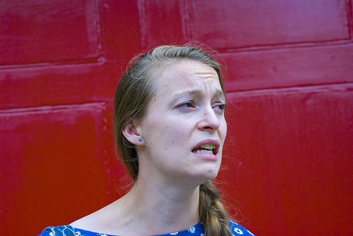
arrbw = np.array(imbw)

The original image in this example looks like this:

The measure of focus that we will use will be the variance in pixel intensity around each pixel location. To calculate variances, we will need some measure of mean intensity at each location and some measure of the mean squared-intensity at the same location. To rapidly iterate through the millions of pixel locations in a typical image, we will calculate values at a location targeted around a particular pixel by using a filter from SciPy’s ndimage module. In order to make sure that the location around the target is not biased in any particular direction, we will use a Gaussian filter, which averages values in an array with decreasing weight on values that are farther from the target pixel. Finally we calculate the variance at each location as the square root of the difference between the square mean intensity (sub_sqr_mean) at each location and the mean intensity squared (sum_mean**2).

sub_mean = ndimage.gaussian_filter(arrbw, sigma)  # Calculate variance in area around each pixel
sub_sqr_mean = ndimage.gaussian_filter(arrbw**2, sigma)
sub_var = np.sqrt(sub_sqr_mean - sub_mean**2)

The array of variances (sub_var) calculated above would be of direct use when comparing the intensity of focus across the same location in a stack of images. However, in this example, we are only concerned with a single image. In this case, to make the variances easier to handle, we scale them all by the largest variance we observe in this image.

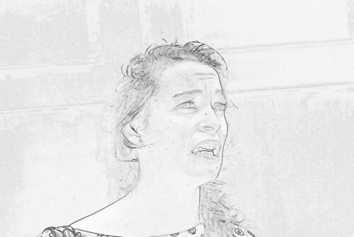
focus = sub_var/sub_var.max() # Define focus at each pixel as scaled variance

Now that we’ve calculated an array of focus values, we can visualise the results by generating some images using it, to check that the array makes sense. One way we can do this is to generate a greyscale image where pixel intensity is the scaled variance (focus) from our original image. While we’re making such a synthetic image, we might as well have a bright background and a dark signal, which is similar to a sketch on paper. To do this we can simply calculate an array where the value at every position [i,j] is 1.0 - focus[i,j]. We can scale these values up to lie between 0 and 255 (the range of signal in a typical greyscale image file) by multiplying each calue by 255.0. Finally we can generate some data which look like an image by rounding the resulting real number to the nearest integer (np.round) and converting resulting values to 8-bit integers (np.array(…,dtype=np.uint8)). With the array is in the correct format, we can use it to generate an image using the Image.fromarray function from PIL.

focus_arr = np.array(np.round(255.0 * (1.0 - focus)),dtype=np.uint8)
focus_im = Image.fromarray(focus_arr)

The resulting image looks like this:

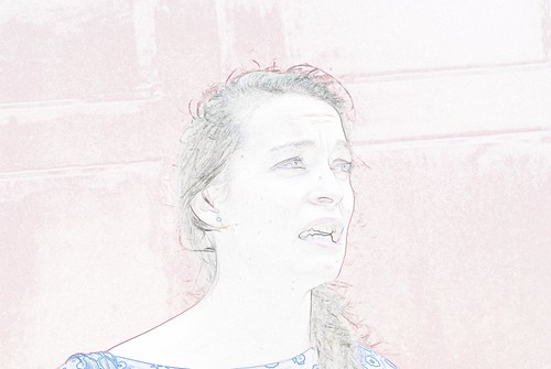
Another way to visualise the focus is the mask the original image using the focus map. This will hide all parts of the original image that are not in focus and recover the original pixel colours for locations that are in focus. Here, you need to choose what background colour to display in the new image where the original is not in focus. Below is an example with a white background. I will not go into the code for generating this mask in detail here, however it is worth noting that there are far more lines of code required for visualisation and image generation than for carrying out the focus calculations.

A complete piece of code for downloading some source images to the working directory from the internet, locating pixels in focus and generating the visualisations mentioned above can be seen in this GitHub gist.

Tags: image analysis image python numpy scipy pil