12 August 2019

Inference for dynamic simulation models

I recently bought a copy of the latest edition of Darren Wilkinson’s book: Stochastic Modelling for Systems Biology because I’m interested to see what he has to say about Approximate Bayesian Computation (ABC).

Browsing through, I am reminded of the very useful example in Chapter 11: Inference for stochastic kinetic Models, which describes a likelihood-free method for Bayesian inference of dynamic simulation model parameters. This approach involves using a bootstrap particle filter for marginal likelihood estimation. Estimating likelihood in this way is a useful component of general inference workflows that can be applied to a wide range of applied models. In 2013, I investigated using this approach to infer parameters from a model of population dynamics by comparing simulation results with experimental observations. I gave a talk about this work (slides here), describing why the biological model and inference problem was interesting, the details of a particular stochastic model of population dynamics (the Discrete Stochastic Logistic Model: DSLM) and an experiment to quantify actual dynamics.

In this post I will describe why you might use this particular type of inference and how you might code it up in a bit more detail. In a later post, I hope to compare this approach with an equivalent ABC workflow.

Bayesian inference

I’m not going to go into detail about why you might prefer to use a Bayesian approach to parameter inference, rather than a frequentist approach. Briefly, for most scientists, the attraction of frequentist analysis is that, in theory, it is objective or unbiased. However, in practice, all parameter inference problems require that you limit your search for a best fitting set of parameters within a tractable parameter space. The choice of search space is an often overlooked source of subjectivity in frequentist analysis. Bayesian analysis is much more up front about subjective, constrained searches of parameter space. You explicitly specify and weight the likely search space by specifying your prior belief about the distribution of model parameters.

From my point of view, the major difficulty with Bayesian inference is making prior beliefs concrete. Statisticians enjoy using distribution models with infinite support: i.e. modelling numbers which can, in theory, take extremely large values. Statistical theory is often built around models with such support. However, interested, practical experimental scientists will, quite rightly, believe that the ranges of parameter values should have realistic constraints. For instance, if you have a parameter which is “mass of micro-organism” and you model your uncertainty about it using the popular Gaussian distribution, you are allowing for a small, but non-zero possibility that the microbe is bigger than your house. You are also allowing for a possibility that it takes a negative value, which is physically meaningless. Whereas, an experienced scientist might put absolute limits on the acceptable range of values to lie between 0 and 1 g.

Software tools and algorithms for statistical computing

There are lots of excellent software tools for Bayesian inference of parameter values for models, given data. Stan, JAGS and pyMC3 are three that I use, for example. Although very useful, these tools are built for statistical modelling and are not so good at handling arbitrary mathematical models. For example, if you want to use JAGS, you have to be able to write your model in the JAGS modelling language. Writing a model in the JAGS modelling language is barely a restriction at all for statistical models, but there are many examples of mathematical models from which it is only practical to simulate using more complete, general purpose programming languages (e.g. C++, Python, Julia, Haskell, Scala, Java). The example in Darren’s book is written in the R programming language. So, here we will consider simulating from models in R, for the moment.

For a given statistical model, it is usually straightforward to calculate the statistical likelihood of a set of data, given a set of model parameters, whereas for mathematical or computational models, this calculation is very often not straightforward. For example, mathematical or computational models can involve numerical solution of differential equations or algorithmic approaches that incorporate intrinsic stochasticity like the Gillespie algorithm or Individual Based Modelling (IBM).

So, likelihood-free methods that avoid this complication are an important approach for carrying out inference for typical mathematical or computational models.

Logistic models of population growth

For this demonstration, we will consider versions of the logistic model: a simple model of how a population grows when resources are limited. Here we will think about modelling populations of cells. We can derive this model in various ways, one way is to think of an irreversible, first order, mass action chemical reaction (Cells + Nutrients → 2 Cells) occurring in a well-stirred vessel. Some details about this way of thinking about logistic growth can be found in the slides from my earlier talk.

Simulating from the logistic model

The deterministic logistic model is a popular tool in ecology and was originally developed to describe the self-limiting growth of human populations. It has an analytic solution which means that it could be used directly in statistical programming languages such as JAGS and STAN. Here is the solution of the logistic model written as a vectorised R function:

# Analytic solution of logistic model of population dynamics
logistic = function(K,r,x0,t) (K*x0*exp(r*t))/(K+x0*(exp(r*t)-1))

If your machine can run the Rcpp package (note, under Microsoft Windows, using Rcpp requires installation of Rtools), you can define a (~20%) faster, vectorised version as follows:

if(require(Rcpp)){
 cppFunction('NumericVector logistic(float K, float r, float x0, NumericVector t){
  NumericVector x = (K*x0*exp(r*t))/(K+x0*(exp(r*t)-1.0));
  return x;
 }')
}

Vectorised function calls are fast in R and writing code to use them is succinct, elegant and similar to how you would describe their use in mathematics. For example, for a given set of parameters K, r and x0, if we pass a vector of times t, we get back a vector x of population sizes corresponding to those times, which we could use to plot the dynamics:

t = seq(0,10,0.5)
x = logistic(K=42.0, r=1.1, x0=1.0, t=t)
plot(t,x,type="b",main="Simulation from logistic model")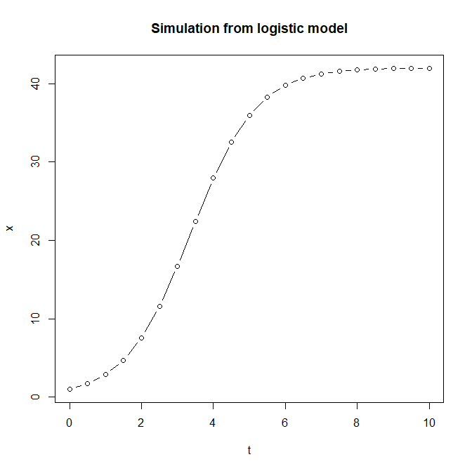

Simulating from the Discrete Stochastic Logistic Model (DSLM):

Simulations from the DSLM are carried out by simulating the dynamics of a small chemical reaction network (described here) using the stochastic Gillespie algorithm. The DSLM simulates all reactions until the nutrient species is exhausted. Unusually for reaction network models, for the DSLM, the total number of “reactions” can be known in advance. This feature allows us to write down the implementation below, which takes advantage of R’s fast vector operations to simulate all reactions at once. Vector notation is great, in that the Gillespie simulation algorithm below is only a few lines long, however it’s also restrictive in that efficient, partial simulation (i.e. simulation only up until a certain time or up to a certain population size) is not really possible, leading to wasted computation in some circumstances. Other programming languages, such as C++ or Julia might allow fast, partial simulation from the DSLM without vectorisation.

# Discrete stochastic simulation of logistic model
# adapted from http://lwlss.net/talks/discstoch/
simDSLogistic=function(K,r,N0){
  if(N0>=K) return(data.frame(t=c(0,Inf),c=c(N0,N0)))
  unifs=runif(K-N0)
  clist=(N0+1):K
  dts=-log(1-unifs)/(r*clist*(1-clist/K))
  return(data.frame(t=c(0,cumsum(dts)),x=c(N0,clist)))
}

Unlike the simulations from the analytic solution of the logistic model above, here we cannot specify values of t at which we would like to know the simulated population size, however the function above returns both t and x for the full simulation, which we can plot in a very similar way:

dat = simDSLogistic(K=42, r=1.1, x0=1)
plot(x~t, data=dat, type="s", main="Simulation from DSLM")

Comparing simulated results from logistic model and DSLM

It’s straightforward to simulate data from both models using the same model parameters and compare outputs. For the parameters chosen below, we can see a wide range of trajectories from the DSLM, centred roughly around the deterministic solution. The range of trajectories represents the intrinsic stochasticity written into the DSLM, which is absent from the deterministic version.

t = seq(0,10,0.5)
x = logistic(K=42.0, r=1.1, x0=1.0, t=t)
plot(NULL,main="Simulations from logistic model & DSLM",xlim=range(t),ylim=c(0,42),xlab="t",ylab="x")
replicate(1000,points(x~t, data=simDSLogistic(K=42, r=1.1, x0=1),type="s",lwd=2,col=rgb(0,0,0,0.05)))
points(t,logistic(K=42.0, r=1.1, x0=1.0, t=t),col="red",lwd=3,type="l")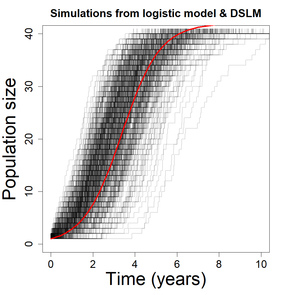

The plot above shows 1,000 discrete stochastic realisations of the DSLM (grey/black) along with the deterministic solution of the logistic model using the same parameters(red). Both models simulating a population which grows to a final size small enough that discrete values taken by DSLM results are clearly visible.

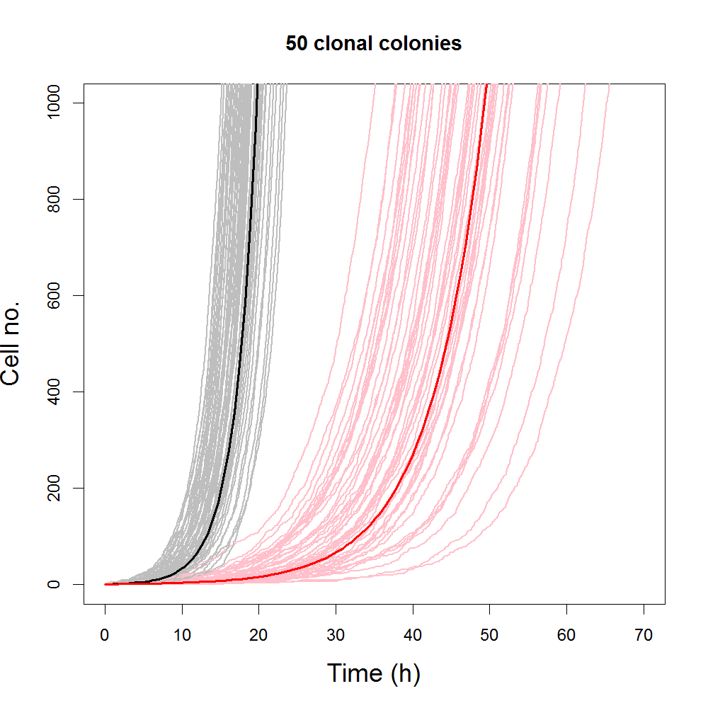
The plot above shows the early progression of simulated population size with time for slow growing populations (red/pink) and fast-growing populations (black/grey). Solid curves are simulations from the logistic model, grey and pink curves are representative ensembles of simulations from the DSLM. Simulations from both the DSLM and logistic model were generated using the same set of parameters. Despite the fact that population sizes simulated from DSLM are large enough that individual curves have very similar shape to deterministic equivalents, individual stochastic simulations are quite distinct from each other. Differences between individual simulations from DSLM are smaller for faster growing population.

Generating synthetic datasets

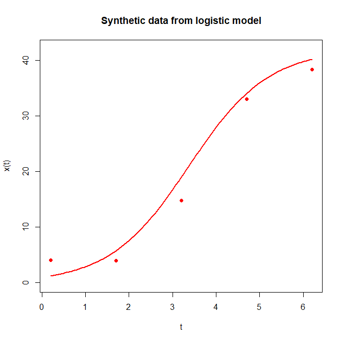
To simulate the process of carrying out an experiment to make some (noisy) observations of population size and in order to be able to know “true” model parameter values, we will work here with synthetic data, generated directly from the model with added noise. Knowing the parameters used to generate these data, we can attempt to use statistical inference to recover the original model parameters from the data. In this way, we save ourselves the effort of carrying out the experiment and provide a means to assess whether our inference algorithms are performing well. However, it’s worth remembering that fitting models to real data and interpreting the fit is much more difficult, since there is an important extra complication: any model is an imperfect representation of reality, so, for real inference problems, as well as dealing with measurement error, there is also model error to consider.

# Generate and visualise synthetic observations (and "true" dynamics) from logistic model
th = c(K=42,r=1.1,x0=1,stdev=2.5)

times = seq(0.2,7,1.5)
dat = data.frame(x = sapply(logistic(th[["K"]],th[["r"]],th[["x0"]],times),function(y) rnorm(1,y,th[["stdev"]])))
rownames(dat) = times

plot(dat$x~times,xlab="t",ylab="x(t)",main="Synthetic data from logistic model",ylim=c(0,th[["K"]]),pch=16,col="red")
newf = function(x) logistic(th[["K"]],th[["r"]],th[["x0"]],x)
curve(newf,from=min(times),to=max(times),col="red",lwd=2,add=TRUE)

The code above generates a plot comparing five synthetic observations (points) with the underlying “true” dynamics (curve) which you can see below:

Inference

To prepare for carrying out this particular inference workflow, we will need a few more functions.

Initial conditions

If our initial condition (in this case, population size at t=0 is not known a priori, then we can learn about it during inference and allow our uncertainty about intital conditions to propagate forward to increase our uncertainty about model parameters. We can specify an informative prior for our initial condition as x0 uniformly distributed between 0 and 1.5:

simx0 = function(n, t0, th) runif(n, 0, 1.5)

Or for the discrete case, something like this, allowing for any x0 ∈ {1,2,3,4}:

simx0 = function(n, t0, th) sample(1:4,n,replace=TRUE)

Step simulations

Next, we will have to make it possible to simulate from our models in a slightly different way: we will simulate from one experimental observation to the next and so need to carry out simulation steps from time t0 to t0 + deltat. We’ll need to specify our model parameters in the form of a vector th rather than separate variables. So, let’s define functions for step simulation for the logistic model:

stepLogistic = function(x0, t0, deltat, th) logistic(th[["K"]],th[["r"]],th[["x0"]],deltat)

Note the function argument t0 is there to make the approach general enough to include models where behaviour depends on time itself. The logistic model and the DSLM evolve in time in a way that only depends on the initial population size, not the starting time, so this argument is redundant for these two models. The step function for the DSLM is a bit more complex, since we have to simulate forward to completion and then go back and find the first model state at which the simulated time is greater than t0 + deltat:

stepDSL = function(x0, t0, deltat, th){
  dsl = simDSLogistic(th[["K"]],th[["r"]],x0)
  if(deltat<=max(dsl$t)){
    dsl$x[which(dsl$t>deltat)[1]]
  }else{
    th[["K"]]
  }
}

Measurement error

We assume that population size is not observed perfectly, but with some uncertainty. Even if this is not really true in practical terms (e.g. if the population is directly countable) then including a measurement error model can be a useful way to account for slight qualitative mismatches between an imperfect model and real data. We can use the same Gaussian measurement error model for both population models, adding a parameter to the vector th representing the standard deviation of the measurement error process: stdev. We can write down the (log-)likelihood of observing some data y at times t, given some simulated results x at times t and our measurement model, parameterised by stdev:

dataLik = function(x, t, y, th) sum(dnorm(y, x, th[["stdev"]],log=TRUE))

Marginal likelihood particle filter

The core of this inference approach is being able to sample from the intractable (log-)likelihood of the parameters th given the data y. The function below gives us a way to access likelihood numerically by particle filter. The function is taken from Stochastic Modelling for Systems Biology, where you can also find a detailed description of why this approach works and how to choose number of particles, for example. It is written as a function closure, a very useful feature from functional programming, whereby one function can return another as output, accessing the local environment of the first function, any time it’s called. In this case, we pass several arguments whose values will remain fixed during inference: n the number of particles, simx0 a function for sampling from the distribution of initial conditions, t0 a starting time for simulation, stepFun a function for simulating from the step version of your model, dataLik a function for simulating from the measurement error model (the likelihood of the data given a simulated result) and data the full set of observed data. The function that is returned depends only on the parameter vector th which we will update often during the inference algorithm.

# pfMLLik
# Particle filter for unbiased estimate of marginal likelihood (logged)
# Adapted from Stochastic Modelling for Systems Biology (3rd Ed.) by Darren Wilkinson

pfMLLik_gen = function (n, simx0, t0, stepFun, dataLik, data) {
  times = c(t0, as.numeric(rownames(data)))
  deltas = diff(times)
  return(function(th) {
    xmat = as.matrix(simx0(n, t0))
    ll = 0
    for (i in 1:length(deltas)) {
      xmat[] = apply(xmat[,drop=FALSE], 1, stepFun, t0 = times[i], deltat = deltas[i], th)
      lw = apply(xmat[,drop=FALSE], 1, dataLik, t = times[i + 1], y = data[i,], th)
      m = max(lw)
      rw = lw - m
      sw = exp(rw)
      ll = ll + m + log(mean(sw))
      rows = sample(1:n, n, replace = TRUE, prob = sw)
      xmat[] = xmat[rows,]
    }
    ll
  })
}

I’ve had to adapt the function above slightly to get around one of many problems with the R language. The original function was written to handle inference for multi-dimensional data and model output (specifically for the Lotka-Volterra model. However, the two logistic models as written above both have one dimensional output: population size. We could, in principle, also attempt to simulate and observe the “nutrients” species from the chemical kinetic formulation of the model, however, those data are not typically captured during population studies. Unfortunately, R does not generalise well from matrix representation of multi-dimensional data to one dimension. By default, R silently converts one-dimensional matrices into vectors: a data type which is not compatible with much of the original algorithm from Stochastic Modelling for Systems Biology. In order to get this function to work for one-dimensional logistic models, adaptations above include typecasting input data as a matrix:

xmat = as.matrix(simx0(n, t0))

and forcing data to remain as a matrix, even when one-dimensional:

xmat[,drop=FALSE]

With the minor adaptations above, this useful function closure can, in principle, be applied to models of and data of any dimension.

Specifying prior distributions

We can specify our vague prior beliefs about the distribution of values of parameters in the vector th, in the form of a prior likelihood for th. Uniform priors are often referred to as “uninformative”, however the uniform priors below are informative since they explicitly specify a range of believable parameter values. In practical terms, when sampling from the uniform distribution, you have to specify informative lower and upper limits (2nd and 3rd arguments respectively in calls to dunif below).

priorlik = function(th){
  pK = dunif(th[["K"]],0,60)
  pr = dunif(th[["r"]],0,5)
  px0 = dunif(th[["x0"]],0,10)
  pstdev = dunif(th[["stdev"]],0,10)
  return(pK*pr*px0*pstdev)
}

Bringing it all together: Metropolis MCMC algorithm

First, we can define a specific instance of the likelihood particle filter:

mLLik = pfMLLik_gen(100,simx0,0,stepDSL,dataLik,dat_dsl)

Next, we can define a function for calculating the value of the RHS of the proportional form of Bayes’ theorem: the product of the prior probability and the likelihood. We will aim to sample from this product as a means to draw samples from the posterior distribution of parameter values, given the model and observed data. Note that it is not worth evaluating this product for combinations of parameter values that we consider unrealistic or physically meaningless (e.g. negative parameter values or sets of parameters where carrying capacity K is greater than initial). So we can check these conditions using a function to test if th fails:

failth = function(th) th[["K"]]<=0|th[["r"]]<=0|th[["x0"]]<=0|th[["stdev"]]<=0|th[["x0"]]>th[["K"]]

and then define a relative probability (RHS of Bayes’ theorem):

relprob = function(th){
  if(failth(th)){
   rprob = 0
  }else{
   rprob = exp(mLLik(th))*priorlik(th)
  }
  return(rprob)
}

We will carry out Metropolis MCMC to access samples from the posterior distribution for parameters th, as described in section 8.4, with example code in section 8.8.2, of Doing Bayesian Data Analysis by John Kruschke (1st edition). The same algorithm is described in section 10.6 of Stochastic Modelling for Systems Biology.

First define nsamps: the total number of samples/MCMC steps to take and burnin: the number of samples to reject from the start of the algorithm, while MCMC settles down to sample from the posterior. Intialise a matrix trajectory for storing samples, including one plausible set of th in the first row of the matrix.

nsamps = 10500
burnin = 500
ndim = 4

trajectory = matrix(0, nrow=nsamps, ncol = ndim)
trajectory[1,] = c(30,2.0,2,4)
colnames(trajectory)=c("K","r","x0","stdev")

Specify a multidimensional proposal function, by specifying the covariance matrix of a N-dimensional Gaussian distribution, where N is the length of th.

sd1 = 7.5; sd2 = 7.5; sd3 = 0.75; sd4 = 0.75
covarmat = matrix(c(sd1^2, 0,0,0,0,sd2^2,0,0,0,0,sd3^2,0,0,0,0,sd4^2), nrow=ndim, ncol=ndim)

Then, we can step through the MCMC algorithm, proposing updates to the current value of th based on our N-dimensional Gaussian (sampling from this distribution requires R’s MASS library), probabilistically accepting or rejecting the update, and moving on to the next MCMC sample. For the DSLM, this can take a considerable amount of time to complete:

for(stepno in 1:(nsamps-1)){
  thc = trajectory[stepno,]
  proposedjump = mvrnorm(1,mu=rep(0,ndim),Sigma = covarmat)
  probaccept = min(1, relprob(thc+proposedjump)/relprob(thc))
  if(runif(1) < probaccept){
    trajectory[stepno+1,] = thc+proposedjump
    if(stepno>burnin) nAccepted = nAccepted + 1
  }else{
    trajectory[stepno+1,] = thc
    if(stepno>burnin) nRejected = nRejected + 1
  }
}

accepted = trajectory[(burnin+1):dim(trajectory)[1],]
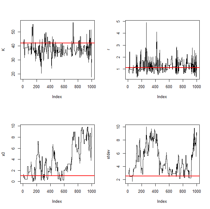
thinned = accepted[seq(1,dim(accepted)[1],length.out=1000),]

Finally we can plot MCMC traces, which we should check for autocorrelation problems that might suggest the algorithm has not yet converged, and posterior density plots:

traceplot = function(param,chain) {
  plot(chain[,param],type="l",ylab=param)
  abline(h=th[[param]],col="red",lwd=2)
}

pRngs = list(
K = c(0,60),
r = c(0,3),
x0 = c(0,10),
stdev = c(0,10)
)

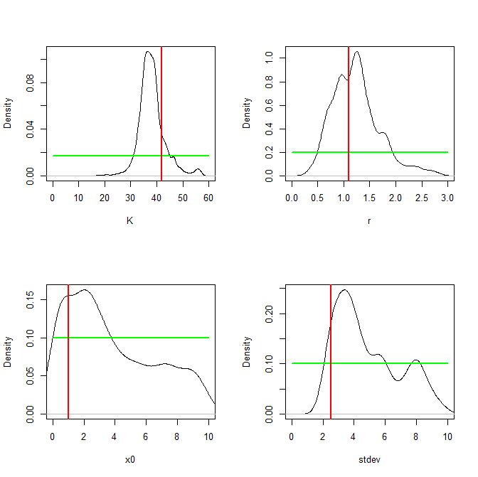
densplot = function(param,chain,pRngs) {
  plot(density(chain[,param]),type="l",xlab=param,main="",xlim=pRngs[[param]])
  pfunc = pfuncs[[param]]
  curve(pfunc,from=pRngs[[param]][1],to=pRngs[[param]][2],col="green",lwd=2,add=TRUE)
  abline(v=th[[param]],col="red",lwd=2)
}

pfuncs = c(
K = function(x) dunif(x,0,60),
r = function(x) dunif(x,0,5),
x0 = function(x) dunif(x,0,10),
stdev = function(x) dunif(x,0,10)
)

op=par(mfrow=c(2,2))
sapply(c("K","r","x0","stdev"),traceplot,thinned)
par(op)

op=par(mfrow=c(2,2))
sapply(c("K","r","x0","stdev"),densplot,thinned)
par(op)

It really annoys me to have to specify separate sampling functions and density functions for plotting priors, basically writing out the same statistical model parameters twice. This seems to be a potential source of serious error! I find myself having to do this with all probabilistic programming languages, however. Anyway, finally, our plots comparing posterior distribution (black), prior distribution (green) and “true” values used to generate synthetic datasets (red) for each parameter are as follows:

Conclusion

This approach is computationally intensive, but extremely general: it can cope with a much wider range of models than statistical modelling tools like Stan and JAGS, in particular it can cope with the kinds of arbitrary dynamic models that are extremely important in general scientific research. However, there are some limitations. I hope to go into these in a subsequent post and to investigate alternative approaches.

You can find the complete R script for running analysis on this page here.