11 October 2017

Quantifying the strength & significance of genetic interactions

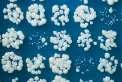
Recently, I have been analysing some functional genomics and drug screen datasets. The techniques I use are similar to those I developed while working on and using a method called Quantitative Fitness Analysis (QFA) (Addinall et al. (2011), Lawless et al. (2010)). QFA is a method for screening the health of up to tens of thousands of microbial cell populations (examples in picture above). It is typically used to search for genes interacting with a gene of particular interest. This kind of genetic screen involves growing a wide range of different, genetically modified cell populations and looking for differences between the observed health of these populations and the health predicted in the absence of interaction.

The first part of a genetic interaction screen using QFA is to evaluate the health of the cell populations under investigation, by examining how each population grows. However, in this article, I want to concentrate on how we measure the strength of interactions and classify populations of a specific genetic type as sufficiently interesting to warrant further investigation. Although the example I present here is from a historical genetic interaction screen, based on QFA, the same statistical and visualisation strategies can be applied to screens with any quantiative output. For example, drug screens, where the output might be the expression of a fluorescent protein in human cells growing in liquid medium.

While developing QFA screens, we created fitness plots: scatter plots for visualising the evidence for genetic interactions when comparing the results from two carefully matched QFA experiments. I have developed an interactive fitness plot designed to make some of the decisions we made about how to interpret QFA screens when looking for interactions clearer. I will present the interactive plot in the next section, before describing how it all works. The plot itself is the most interesting thing, but the description of its various parts will likely be quite long! However, for most readers, the next section will make more sense if it is read after the rest of the article. You can also just skip to the conclusion.

A Quantitative Fitness Analysis (QFA) fitness plot

The two genetic screens in this example were published in Addinall et al. (2011), which was the first scientific article to describe QFA, and were designed to identify genes interacting with CDC13. CDC13 is a gene that codes for a protein called Cdc13 which plays an important role in stabilising eukaryotic telomeres. Telomeres are structures that prevent our strands of DNA from unravelling in the same way that plastic ends stop our shoelaces unravelling. cdc13-1 is a mutant allele of the CDC13 gene that codes for a temperature-sensitive version of the Cdc13 protein: Cdc13 produced by cdc13-1 is defective when cells are grown at temperatures above ~26°C, but works normally at lower temperatures. The screens presented in the fitness plot above were carried out at 27°C in order to cause a fitness deficiency in strains from the cdc13-1 screen that is detectable by QFA.

In this interactive fitness plot, changes you make to Fitness summary, Fitness definition, Significance cutoff and Type of model fit, by adjusting the values in the boxes above the plot, are reflected in the plot in real time. The fitness definition is updated, the raw fitness data are re-summarised, the model of genetic independence is recalculated, the statistical significance of any genetic interactions are recalculated and then the plot is redrawn with appropriate axis scales.

We have previously developed a related interactive fitness plot tool called DIXY for comparing between QFA experiments. In contrast, this version is for comparing the effect of QFA design choices on estimates of genetic interaction within a single QFA experiment.

Quantitative Fitness Analysis (QFA)

QFA is an experimental & computational method for measuring the health of populations of microbial cells. High-throughput QFA is often carried out with the assistance of laboratory robots to screen the health of libraries of tens of thousands of different genetically modified cell populations. The aim of these screens is typically to uncover evidence for previously unknown interactions between genes. A genetic interaction is said to occur when the effect of one gene on some characteristic (or trait) of the population is dependent on the presence of one or more other genes. Identifying genetic interactions, in carefully chosen genetic backgrounds and under carefully controlled and constant environmental conditions, gives us clues for how gene products (e.g. proteins or protein complexes) interact within living cells.

Evolutionary fitness is a quantitative measure of a population’s success during natural selection. Fitness is the average, expected contribution to the gene pool of the next generation that is made by individuals from the specified population. Fitness is a uniquely informative characteristic (or phenotypic trait) of a population: a direct measure of population health. A population of living organisms cannot tolerate a reduction in evolutionary fitness lightly. Populations with low fitness would be rapidly out-competed during natural selection in the wild.

A major component of the fitness of microbial cells grown in the lab is the rate at which cells divide (population growth rate); fast-growing populations consume limited nutrients more quickly than competing populations and become more abundant over identical time periods. Much of the work in QFA is about generating robust, quantitative estimates of growth rate as a surrogate measure of fitness. However, QFA also measures other aspects of cell growth. QFA is fundamentally about generating growth curves: measuring the increase in population size (or population cell density, see figure above) over time. One thing we can do with a growth curve is to use it to estimate the growth rate of cell populations during the exponential phase, where the effects of nutrient limitations (competition within populations for nutrients) and competition between populations for nutrients are at a minimum. However, another component of fitness is the carrying capacity of the population: how large can the population grow given a finite amount of nutrients? In principle, carrying capacity tells us something about how efficiently the population converts nutrients into cells and is a component of evolutionary fitness. In practise, during QFA experiments, where competition between populations for limited nutrients is likely to become significant at some point during growth, final population size is likely influenced by growth rate during exponential phase and the relative growth rate of neighbouring populations. Populations are likely achieve large final cell densities largely because they competed more successfully with neighbouring populations for nutrients during the early phases of growth by growing more quickly.

By fitting a growth model (e.g. the logistic model) to growth curves, we can choose to examine growth rate as a fitness trait on its own, or to combine growth rate and carrying capacity (e.g. MDRMDP fitness measure from Addinall et al. (2011)). We can also choose to ignore model-based measures of fitness entirely and concentrate on the growth curve itself. One way to do this is to look at the Area Under the growth Curve (AUC). This is another way to combine growth rate and final population size: choose an arbitrary time to truncate growth curves and use the area under the truncated curve as a measure of fitness. The main difficulty with the AUC approach is how to choose the arbitrary truncation time.

Measuring quantitative fitness traits allows us to compare fitnesses between populations; we can use statistics to search for interesting, reproducible differences in fitness. Statistical tests for reproducible differences in fitness form the basis of genome-wide genetic interaction screens.

All phenotypic traits, including fitness depend on genotype. Understanding the connection between genotype and phenotype is an important part of biological research and that is the goal when searching for genetic interactions using QFA. Fitness also depends on environment, which can change rapidly with time in the wild. When cells are grown in the laboratory, extra care is taken to ensure that the environment experienced by cells during QFA is reproducible. For example, cells are grown in humidity and temperature controlled incubators, isolated from fluctuations in the lab. Although cells are provided with the same level of nutrients initially, QFA cell populations take their nutrients from the finite agar substrate on which they’re grown. This substrate becomes exhausted after the cell populations have grown for a few days. This means that environmental nutrients are not constant with time, but ideally nutrient availability is the same for each population. However, since hundreds of independent populations are grown on the same agar substrate, there remains the possibility that fast-growing populations can out-compete slow-growing neighbouring populations by consuming nutrients from their shared pool in the substrate more quickly. During QFA we often design experimental conditions so that we can assume this effect is negligible, especially at the start of the experiment. For experiments where this kind of design is not possible, competition effects in QFA experiments could be explicitly accounted for by simulation modelling work (Boocock & Lawless (2017)).

QFA continues to be used for biological research, for example some QFA screens were published in G3 this year (Holstein et al. (2017), Makrantoni et al. (2017))).

Measuring genetic interaction by comparing QFA screens

On a practical level, genome-wide QFA screens take a considerable amount of time and effort to complete. They are typically carried out in sections, over several weeks. It is challenging, but critically important, to ensure that the environment experienced by each of the strains in both of the screens is comparable. This allows us to ascribe any fitness differences (or interactions) we observe to genetic differences alone and specifically not to environmental differences. It is interesting to note that these challenges are considerably reduced when carrying out QFA on a smaller scale (as discussed by Banks et al. (2012)).

Genetic interaction strength

We search for genes interacting with a gene of interest yfg by carrying out two separate, genome-wide QFA screens. The first, control screen, measures the fitness of each strain in a library of genetic disruptions (e.g. the yeast knock-down library, containing ~5,000 deletion strains each of which is missing one of ~5,350 genes in the yeast genome). I will use xyzΔ as a placeholder for any one of the control deletion strains from the knock-down library. The second, query screen, measures the fitness of the same library, but this time each strain is combined with a disrupted version of the gene of interest (e.g. a deletion, like yfgΔ or some other disruption, like cdc13-1 in the fitness plot above). We use the observed fitness of the single mutant xyzΔ strains (which we denote [xyzΔ]) to predict the fitness of each of the double mutant yfgΔxyzΔ strains, assuming no genetic interaction. We predict fitnesses using Fisher’s multiplicative model of genetic independence, which says that, in the absence of interaction:

$$\frac{[yfg\Delta xyz\Delta]}{[wt]} = \frac{[yfg\Delta]}{[wt]}\frac{[xyz\Delta]}{[wt]}$$

Where wt is a wild-type strain (i.e. [wt] is the fitness of a strain with no genetic modifications, in identical environmental conditions, or a good surrogate for it). Fisher’s model mirrors a calculation from probability theory: the probability that both of two independent events occur, given their individual probabilities. This model applies to any quantitative phenotypic trait, not just fitness. The terms in the model can be rearranged to make the predicted relationship between query screen fitnesses ([yfgΔ xyzΔ]) and equivalent control screen fitnesses ([xyzΔ]) explicit:

$$[yfg\Delta xyz\Delta] = \frac{[yfg\Delta]}{[wt]}[xyz\Delta]$$

We carry out QFA of multiple independent replicates of each strain to allow statistical analysis to assess whether differences between observed [yfgΔ xyzΔ] and predicted [yfgΔ xyzΔ] assuming no interaction, are significant. Given considerable levels of biological heterogeneity and the difficulty of controlling technical error in high throughput experiments, I recommend at minimum eight replicates per strain.

In order to make the prediction (i.e. in order to evaluate the RHS of the equation) we to need estimate the $\frac{[yfg\Delta]}{[wt]}$ term above. There are two ways we can do that: 1) measure [yfgΔ] and [wt] directly, bearing in mind that these values are critical for identifying interactions, therefore many extra replicate strains should be investigated, or 2) estimate $\frac{[yfg\Delta]}{[wt]}$ by fitting a linear regression model through the origin and each of a large, unbiased collection of strains, the overwhelming majority of whom we can safely assume do not interact with the query strain. These two options are available for exploration in the fitness plot above by choosing Type of model fit as either 1) Regression or 2) Wild-type.

Statistical significance of observed interactions

There are several options for assessing the statistical significance of interactions. The most straightforward, practical option is to carry out Student’s t-tests for whether the mean of observed [yfgΔ xyzΔ] is different from predicted [yfgΔ xyzΔ], giving a p-value for each xyz. This t-test approach is automatically applied when you select mean as the Fitness summary in the fitness plot above. An alternative approach is to test whether the median of observed [yfgΔ xyzΔ] is different from predicted [yfgΔ xyzΔ] using the Mann-Whitney U test, again giving a p-value for each xyz. This Mann-Whitney approach is automatically applied when you select median as the Fitness summary.

In any QFA experiment to identify genetic interactions (but especially genome scale experiments), either of these approaches will result in issues with multiple-testing which must be addressed. As in Addinall et al. (2011), here I apply False Discovery Rate (FDR) corrections to the list of p-values to generate a list of corrected q-values. We then apply the Significance cutoff to the FDR-corrected q-values.

An alternative to the two approaches above is to apply ANOVA to measure significance of results. I do not recommend this approach as it achieves statistical power by making the strong assumption that all strains have a common variance (and fitnesses are normally distributed). This reduces the likelihood of making Type I error, but actually, in noisy genomics screens with few replicates, Type II error is the real enemy. Following up hits from screens is labour-intensive and expensive. During genomics screens we should concentrate on robustly identifying strong hits and accept that we may miss some true but weak hits. Pair-wise testing with correction for multiple comparisons achieves this aim. Real screen data often include few replicates and strong outlier observations that are not captured well by the normal distribution underlying ANOVA.

A far better alternative to ANOVA lies somewhere between the two extremes: share information between strains, but do not insist that all strains have the same variance. We can achieve a compromise here by using Bayesian inference for a hierarchical model of variance, as carried out by Heydari et al. (2015). The most advanced approach presented by Heydari et al. includes fitting logistic population models to growth curves within the hierarchy for more powerful inference of logistic model parameters. Although attractive, the computational cost of this approach remains prohibitive. However, Bayesian hierarchical modelling of fitnesses to infer genetic interaction can be completed in a matter of hours, and is a practical offline alternative.

QFA fitness plots

QFA fitness plots are tools for visualising the evidence for genetic interaction when comparing two QFA screens. Where possible, the conditions of the experiment should be designed so that points on the fitness plot lie roughly half-way between the x-axis and the line of Equal fitness. This allows equal space above and below the line of Genetic independence for identifying suppressors (blue points) and enhancers (red points) of the query mutation (cdc13-1 in this case). Vertical distance of each point from the line of Genetic independence is a measure of the strength of genetic interaction. Coloured points indicate that the genetic interaction is estimated to be reproducible, not a random artifact (i.e. statistically significant).

QFA fitness definitions

QFA generates several different quantitative fitnesses from observed growth curves. Each have their advantages and disadvantages as surrogates for evolutionary fitness. It is worth thinking carefully which is the most appropriate for each pair of experiments.

r

Growth rate parameter estimated after fitting the logistic model to the population growth curve. r represents the intrinsic growth rate of the population in the absence of any nutrient constraints and is closely related to evolutionary fitness.

K

Carrying capacity parameter estimated after fitting the logistic model to the population growth curve. K represents the final population size and in the absence of competition for nutrients, is a measure of how efficiently a population can make use of limited resources. In QFA, where competition effects are sure to become important at some point during the growth curve, it is likely that K, the population size at the end of the experiment, is strongly affected by growth rate earlier in the experiment. Faster growing strains utilise shared nutrient pools more quickly, depleting them and reducing availability for their neighbours.

MDR

Maximum Doubling Rate: rate at which population is doubling at the start of the experiment (assumed to be the maximum rate). Described in detail by Addinall et al. (2011).

MDRMDP

Maximum Doubling Rate * Maximum Doubling Potential: dimension-matched product of growth rate and carrying capacity used as fitness measure in Addinall et al. (2011).

nAUC xxx

A numerical (i.e. model-free) estimate of area under the growth curve up to xxx days after inoculation. A range of different values of the arbitrary cutoff xxx are included so that you can see how the performance of this measure of fitness changes in with cutoff.

Fitness summary

Static fitness plots for the model organism S. cerevisiae (brewer’s yeast) typically include ~5,000 points, corresponding to average fitness of individual deletions of most of the ~5,350 genes in the S. cerevisiae genome. This is already quite a lot of data to think about, but actually, each of these points summarises several replicate measurements made in two independent genome-wide screens. Measurements should be well replicated (a minimum of eight replicates per genotype) to capture experimental error and biological heterogeneity. With eight replicate measurements in each of two screens of ~5,000 genetically modified strains, that amounts to 80,000 fitnesses in a single plot. In the interactive fitness plot at the top of this article, hovering over any summary point displays vertical and horizontal lines indicating the replicate values in each of the screens.

Mean

Represents the expected value of a further observation. When mean is selected as the summary statistic, then the statistical significance of deviations from the model of genetic independence are estimated using Student’s t-test.

Median

Represents the value at which the observed dataset is split in two. Does not depend on assumed statistical distributions. Median summary is often one of the samples themselves. This feature is important because it allows us to precisely detect fitnesses that are exactly equal to zero. Synthetic lethal genetic interactions are those which kill the cells (giving them a fitness of exactly zero, in reality). It is very useful and reassuring to be able to clearly identify synthetic lethal interactions in the context of a quantitative screen. When median is selected as the summary statistic, then the statistical significance of deviations from the model of genetic independence are estimated using the Mann-Whitney U test.

Max & Min

Maximum and minimum replicate values respectively. Not recommended as a useful summaries.

Significance cutoff

Probability, under the null hypothesis, of obtaining a hit as strong or stronger than that actually observed if you repeated the experiment. Hits are classified using False Discovery Rate (FDR) corrected p-values (also called q-values). Since the cutoff is a probability, it should be a real number between 0.0 and 1.0. Genes with a q-value below this cutoff are classified as showing statistically significant interaction with the query mutation. Traditionally, in biology, a cutoff of 0.05 is used, but this value is completely arbitrary. It’s worth noting that statistical significance does not guarantee biological significance, but rather is an indication that further investigation is justified.

Type of model fit

Regression

The slope of the line corresponding to Genetic independence is estimated by linear regression (through the origin) through all ~5,000 summary points.

Wild-type

The slope of the line corresponding to Genetic independence is estimated by direct observation of many replicate wild-type strain fitnesses in each of the two QFA screens.

Conclusions from interacting with the fitness plot

Switching between different fitness definitions, we can see that some perform better than others. Using growth rate r as our fitness definition most points lie below the line of equal fitness and points are nicely situated half-way between the x-axis and the line of Equal fitness. Having points below the line of equal fitness is consistent with the query mutation inducing a fitness defect. We usually do not expect any strains with a fitness defect to be fitter than those without a fitness defect. Having points lying half-way between the x-axis and the line of Equal fitness allows the same opportunity to identify both suppressors and enhancers of the fitness defect induced by the query mutation. In contrast, carrying capacity K has neither of the positive features outlined above. More worryingly, the order of genetic interaction strengths is quite different between r and K. K can be dominated by the effects of competition between neighbouring strains during QFA and is not a great measure of fitness in this context. MDR and MDRMDP fitness plots are quite similar to r. MDRMDP is a fitness measure that was introduced by Addinall et al. (2011) as a way to try to extract extra information from the K parameter. An alternative, albeit computationally challenging, approach to extract information from observations of K during QFA is to model competition explicitly (Boocock & Lawless (2017)). The nAUC fitnesses listed are quite good at identifying believable suppressor interactions, even when truncating growth curves at relatively early timepoints. At later timepoints, a large proportion of nAUC fitness estimates end up above the line of Equal fitness (indicating that these, too are probably affected by competition), however, unlike K, the order of interactions remains plausible and similar to that of r. It’s worth noting that it other QFA experiments, which are carried out with higher starting populations, nAUC performs well as a measure of fitness (Dubarry et al. (2015)).

Varying the fitness summary statistic from mean to median, we can see that differences are minor, except that, when using median, it is possible to identify strains whose fitnesses are exactly zero. This is especially useful for identifying so-called synthetic lethal interactions: genes whose deletion in combination with the query mutation, completely kill cells. Synthetic lethal interactions are of particular interest to many researchers. I don’t think there are any good examples in the screens presented here, but if your results include occasional extreme outliers, the median summary is far more robust to those than the mean.

Using the default settings above, we can identify hundreds of genes displaying interactions with cdc13-1 that are statistically significant, which should be investigated further. Choosing a lower cutoff for statistical significance results in fewer hits, as expected. In biology, it is traditional to use a cutoff of 0.05. However, this value is arbitrary. It’s interesting to note that, even when reducing the cutoff by an order of magnitude (to 0.005), dozens of significant suppressors and enhancers are still identified in this screen. The results from this experiment suggest that there is a huge network of genes interacting with the query mutation cdc13-1. On the other hand, most biology experiments and articles in biological journals, focus on individual interactions or a very small number of interactions in great detail. Screens like this one suggest that, despite the structure of the biology literature and successful biological research careers, genetic interaction networks are extraordinarily complex. It does not seem likely that, in cases like this, single-gene, reductionist approaches will lead to complete answers for even quite focused questions about biological function.

Finally, we can see that for most combinations of fitness definition and fitness summary, the choice of whether to estimate the slope of the line of Genetic independence by linear regression through a large, un-biased dataset (as in Addinall et al. (2011)), or through direct observation of extra replicates of wild-type strains in both QFA screens, is unimportant in this example. Switching between the two types of Model fit results in changes in the model of Genetic independence that are barely noticeable and correspondingly small effects on the number and type of significant hits identified. This is an important observation, because the wild-type method allows the design of cheap, high-quality, QFA experiments at sub-genomic scales that can still utilise all the statistical power of QFA screens to identify genetic interactions without specialised, expensive high-throughput equipment.