01 January 0001

When should a dynamic model also be stochastic?

I work in the Wellcome Centre for Mitochondrial Research at Newcastle University. Our research focusses on mitochondria, which are organelles present in each human cell that are primarily responsible for producing the energy that supports cell function. Mitochondria are very important: cells need energy to thrive and they are very unusual: they contain many copies of their own small, circular, multi-copy genome or mitochondrial DNA (mtDNA). mtDNA is independent from their more famous cousins the linear DNA found in the nuclear chromosomes of each cell.

The instructions for how to build the vast majority of molecules produced in the cell, including those that make up the mitochondria, are found in linear, nuclear chromosomes. However, a small number of mitochondrial proteins and t-RNA molecules are assembled according to instructions written in mtDNA. Mutations in mtDNA can affect mitochondrial function and, in particular, cell energy production by the respiratory chain. Mutations in mtDNA are a major cause of mitochondrial disease. Germ-line mtDNA mutations can be inherited maternally, causing mitochondrial disease to run in families.

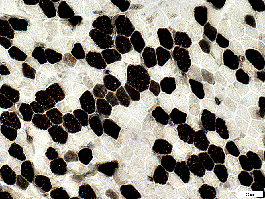
Since there are many (up to thousands) copies of mtDNA in each cell, in contrast with only two copies of each linear DNA chromosome in the nucleus, the propagation of any mutations that arise in mtDNA molecules within a single cell can be extremely complex. This complexity is reflected in the random outcome of some forms of mitochondrial disease. Typically some tissues are affected in patients more than others and the affected tissues can vary from patient to patient. A more concrete demonstration of the random nature of mitochondrial disease is the so-called mosaic pattern of respiratory chain deficiency which is seen in cross-sections from skeletal muscle biopsies taken from patients with some forms of mitochondrial disease. Here we see some skeletal cells affected by disease (dark) and nearby cells, even direct neighbours, completely unaffected. This spatially random pattern suggests that some process is going on independently inside each individual cell individually that can rise to deficiency.

It is known that there is a connection between certain types of mtDNA mutation and biochemical deficiency. However, the proportion of mutant mtDNA molecules in a cell (mutation load) has to exceed an effective threshold before a biochemical deficiency is observed. An interesting and largely open question in mitochondrial research is: by what process does mutation load reach such high levels? This is an important question for understanding the progression of mitochondrial disease. mtDNA does not have the same sophisticated error-checking and repair mechanisms that nuclear DNA has, so the random appearance of de novo mutations in mtDNA is not unusual. However, mutation of one mtDNA molecule results in a very low mutation load, since there are as many as 10,000 molecules in total within a cell. Whereas cells can be found with mutation loads as high as 95%, where, importantly, all mutations are the same. The existance of these almost clonal populations (almost total homoplasmy) suggests that mutations have expanded somehow from a starting population of one. mtDNA mutations can be inherited maternally, but inherited mutation load can be quite low and yet sometimes children suffer under the burden of a very high mtDNA mutation load in some or all of their tissues.

A lot of my time is spent thinking about the population dynamics of mitochondrial DNA (mtDNA) in the progression of mitochondrial disease and in normal human ageing. A popular theory about clonal expansion of mtDNA mutations is that it proceeds by random/neutral genetic drift.

Random outcomes and stochastic processes.

Random vs deterministic.

Stochasticity and selection.

The simplest type of autoregression model, the so-called AR(1) process, is interesting as a model flexible enough to include both one dimensional Brownian motion and white Gaussian noise as special cases. An AR(1) process is plotted above. You can change the model parameters $\alpha$ and $\sigma$ (both described below) using the sliders beneath the plot. Similarly, you can zoom in to or out of the start of the process using the “Horizontal zoom” slider.

During Bayesian inference by Gibbs sampling, for example, we often need to investigate chains of MCMC output. It is important to verify that there is no correlations within these MCMC chains before assuming that samples from the chains correspond to unbiased samples from the posterior distribution. One way to do this is to treat the chains as time series, to plot these and then to visually check the resulting dynamic process for evidence of autocorrelation. Visual inspection of simulated output from AR(1) processes can help us to build an intuitive sense for whether a stochastic time series is autocorrelated.

AR(1) is a stochastic process $X$ varying with discrete time $t$, where the value of $X$ at time $t$ (written $X_t$) is proportional to the previous value ($X_{t-1}$), adjusted by the addition of a noise term ($\epsilon_t$). $\alpha$ is the constant of proportionality and it controls the degree of autocorrelation in the process:

$X_t = \alpha X_{t-1} + \epsilon_t$

where $\epsilon_t \sim N(0,\sigma)$

A sensible algorithm to simulate $t_{max}$ steps from $X$ would be to start off by defining $X_0$ and then, for each subsequent $t \in 1,…,t_{max}$, use your computer to generate a (pseudo-)random value for $\epsilon_t$, and use that to generate $X_t$, following the expression above. Some example Python code:

import random

alpha = 0.5
sigma = 1.0
tmax = 100
X = [None] * (tmax+1)

X[0] = 0
for t in range(1,len(X)):
  X[t] = alpha * X[t-1] + random.gauss(0,sigma)

Another way to do the same thing is to generate and store some random samples from the Gaussian distribution separately, then use the same random samples to explore the effect of different values of $\alpha$ or $\sigma$. This way allows the generation of the plot above, where we can explore what the AR(1) process looks like for different values of $\alpha$, all other values being the same:

import random

tmax = 100

eps = [random.gauss(0.0,1.0) for x in range(0,tmax+1)]

def simulate(eps, alpha = 1.0, sigma = 1.0):
  X = [None] * (len(eps))
  X[0] = 0
  for t in range(1,len(X)):
    X[t] = alpha * X[t-1] + sigma * eps[t]
  return(X)

X_brownian_motion = simulate(eps, alpha = 1.0, sigma = 1.0)
X_white_noise = simulate(eps, alpha = 0.0, sigma = 1.0)

A third way might be to accept that computers are completely deterministic machines and that the random numbers your favourite software tool generates are, in fact, pseudo-random and completely reproducible. However, I won’t go into this now, I will probably write another short post about this issue soon.

It’s interesting to think about what would happen if $|\alpha|>1$. In this case, the process becomes dominated by exponential growth (a kind of numerical explosion!) which rapidly becomes much greater in magnitude than the noise component. In this case the resulting process is no longer obviously stochastic, and so not really AR(1). As such, I’ve restricted the adjustable range for $\alpha$ in the interactive plot above so that it lies between $0$ and $1$.

Much of the interesting changes in shape that take place while varying $\alpha$ occur for values very close to $1$. To highlight that, I have applied a nonlinear transformation between the slider position and the value of the $\alpha$ parameter used to draw the plot. Note that the actual $\alpha$ parameter value is reported at the top of the plot.

Setting $\alpha = 1$ recovers highly autocorrelated one-dimensional Brownian motion (the so-called Weiner process). Setting $\alpha = 0$ gives completely independent samples from the Normal distribution (white Gaussian noise). It’s interesting to note that, by eye, it is quite difficult to differentiate between the process generated when $\alpha$ is as high as 0.5 and that when there is no autocorrelation ($\alpha = 0$). It might be worth bearing this in mind when visually inspecting MCMC output for correlation.