In part I of this series of posts, I presented the mathematics behind circle packing. In part II I demonstrated an implementation of this problem in R, together with an R function for visualising candidate solutions. In part III I tested some optimisation algorithms from various R packages.

In this post I will present an implementation of this problem in Python (code below), a first attempt at optimisation with the same L-BFGS-B algorithm (local optimisation subject to boundary constraints, this time from the scipy.optimize package) presented in part III and some functions for visualising solutions with Scalable Vector Grapics (.svg files).

I generally prefer writing code in Python to R. Python is a more "proper" programming language, is more flexible and extensible than R and has more beautiful syntax and is therefore more readable (which is particularly important when you write code as messily as I do).

R does have some advantages. Its package system (for extending and documenting R functionality) is extremely easy to use and efficient. Data frames in R are versatile, spreadsheet-like objects allowing you to mix different types of data (e.g. text, integers, real numbers) and label data with strings (names of rows and columns). There is no equivalent in Python or other programming languages. R handles plotting, in a flexible, dependable way (requires an external package in Python).

Theoretically, Python should be faster than R, but while writing the code below, I was surprised to find that accessing elements of NumPy arrays using square bracket [] notation was approximately 3 times slower than the equivalent vector operations in R. Fortunately I had read this post about numpy.take (cheers Darren!) which speeded up access by a factor of 3, rendering objective function evaluation speeds approximately equal in both R and Python. I am still quite surprised that they are not significantly faster in Python.

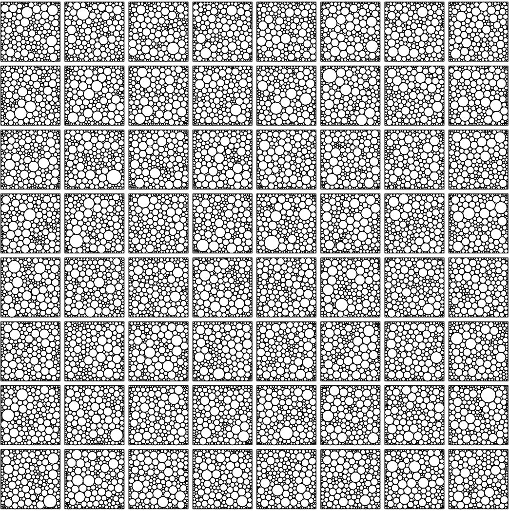
In part II I presented the drawCircles R function to visualise circle packing solutions. I am quite happy with this, particularly because it produces vector graphic output (in the form of a .pdf file). However, it's not perfect. For one thing, I had to convert the .pdf to a .png file to display the image online.

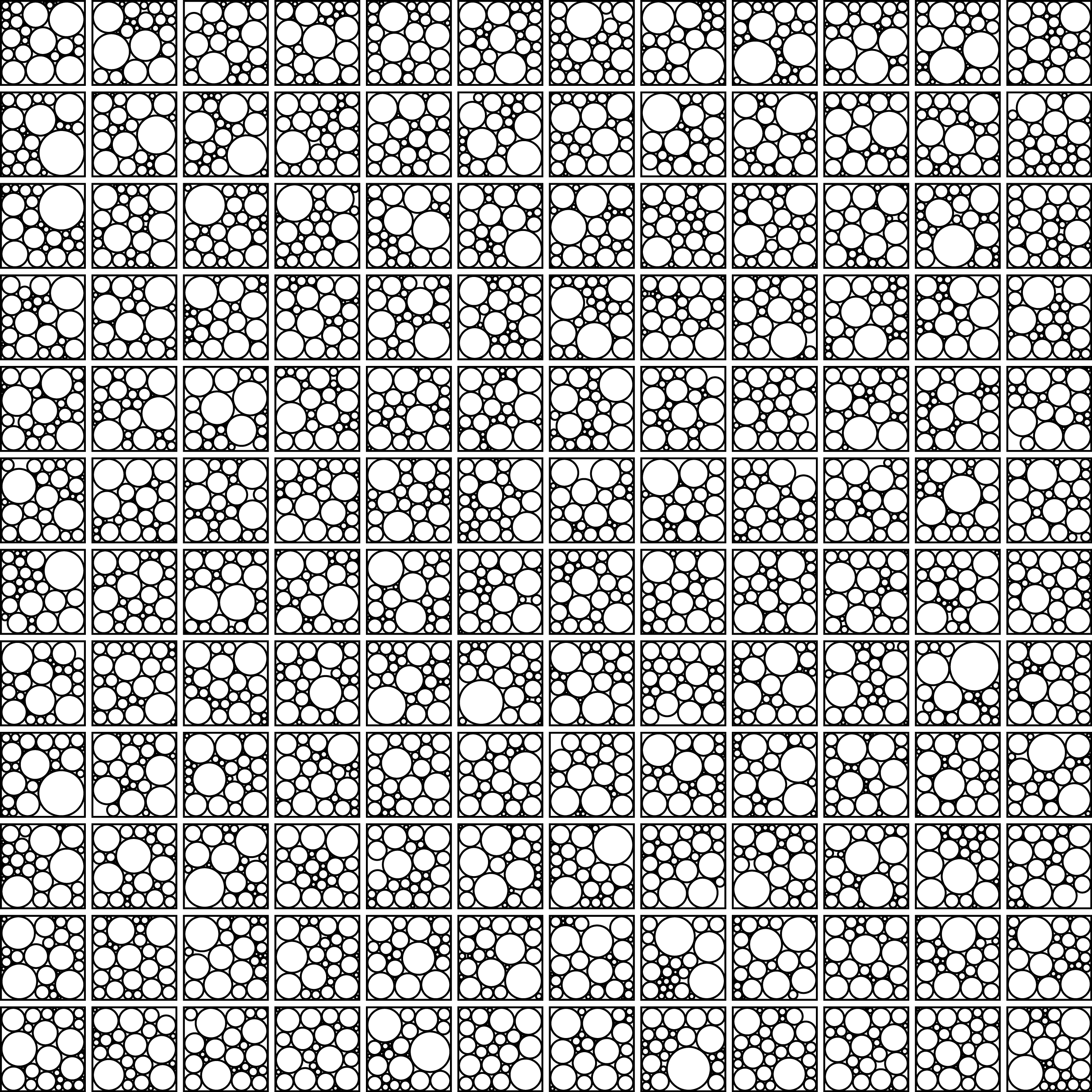
For the Python equivalent, I no longer have access to native plotting functions, but can trivially use Python to build up text files to draw graphics. I have been a fan of manually writing PostScript files for a long time (I am a proud owner of a copy of Adobe's Blue Book), but for this example I chose to try out svg. I don't yet know if svg is as powerful as PostScript, but it is more straightforward for creating images of arbitrary size and aspect ratio with svg (no longer constrained by physical page sizes). SVG is a vector graphics format which can be converted losslessly to PostScript or pdf. SVG is a native web format, so I can display output images online directly like this.

Unfortunately Drupal (the CMS I use to run this blog) doesn't yet allow embedding of .svg images. I haven't been able to get John Flower's SVG module to work (I probably need to upgrade my installation of Drupal). As far as I can tell, WordPress suffers from the same difficulties with svg as Drupal. Something to watch out for when choosing a tool for posting online... I would really rather have something which serves up standard .html. Here is the raster image version of the original:

Finally, here's the code. It uses the NumPy package to allow building and manipulating of arrays and the numpy.take trick mentioned above to speed up accessing elements. It also uses a function closure to define the objective function for comparison with the R equivalent from part II.